Tribology is the study of the friction, lubrication, and wear of interacting surfaces in relative motion. This article explains what a tribosystem is and describes the different types of friction and wear that affect these tribosystems as well as how lubrication can reduce these affects. It also focuses on methods to test and evaluate tribological behavior implemented on tribometers.
Basics of tribology
What is tribology?
The term “tribology” was coined by Sir Peter Jost in 1966[1]. It is derived from the Greek word tribos, which translates to “I rub” in English. Tribology is an interdisciplinary topic involving various branches of science and technology, such as mechanical engineering, material science, physics, chemistry, biology, and food science. Conventional tribological investigations deal with the study of efficiency, performance, and longevity of engine and machine components. However, over the past few decades, it has also proven to be an important tool to characterize different applications ranging from hard disks to skin creams, haptics, prosthetics, implants, food, and beverages.
What is a tribosystem?

Figure 1: Tribosystem
In rheology, which is the science of flow and deformation behavior of materials, the sample’s intrinsic properties are investigated with respect to external influences. In tribology, however, the behavior of the entire tribosystem is studied. The tribosystem comprises of the mating surfaces and the lubricant (when present), as shown in Figure 1.
Dry tribosystems, as the name suggests, are those which have no lubricant between the mating surfaces, such as:
- tire and road
- finger and smart phone
- shoe sole and floor
Lubricated systems, on the other hand, consist of two mating surfaces with a lubricant in-between. Examples of lubricated tribosystems are:
- systems comprising of nib/ink/paper
- cartilage/synovial fluid/cartilage
- eyelid/tear film/cornea
- gear flank/gear oil/gear flank
The performance of a tribosystem is influenced by many factors such as temperature, roughness and surface conditioning of the mating surfaces, humidity, contact pressure, relative velocity, and type of motion. It is possible to simulate the behavior of a tribosystem on a tribometer.
Types of friction and the coefficient of friction

Figure 2: Friction blocks
Friction is the force opposing motion between two surfaces. REF _Ref40850794 \h Figure 2 depicts a simple scenario in which the upper body (Body 1) is sliding against the lower body (Body 2). Here, a force FN is acting on Body 1 in the direction perpendicular to the plane of contact. This force is also called the normal force. On the other hand, friction force FF is the force opposing the motion and it is acting in the opposite direction of motion. The ratio between the friction force and the normal force is called the coefficient of friction. It is a dimensionless quantity denoted by the Greek alphabet µ (mui). Friction is not an inherent property of the material but is a characteristic of the entire tribosystem.
There are three different types of friction, i.e., static, kinetic, and rolling friction. Their corresponding friction coefficients are denoted by µs, µk, and µr, respectively, and they usually follow the following order: $$ µs, > µk, > µr$$
Static and kinetic friction

Figure 3: Block sliding on an inclined plane
As the name suggests, static friction is the friction experienced by two surfaces which are not in relative motion. The easiest way to imagine static friction is to assume a block resting on an inclined plane, see Figure 3. Here, one component of the gravitational force, mg sinθ, is acting towards sliding this block down the plane. This, however, is being inhibited by the frictional force f acting in the opposite direction. The block only begins to move when mg sinθ is greater than f. Up until this point the friction experienced by the system is the static friction. The moment the block starts to slide, we would be looking at the kinetic friction of the system. The friction coefficient corresponding to this transition point is the limiting friction of the system.
Types of wear
Wear is the alteration of a solid surface by progressive loss or progressive displacement of material due to relative motion between that surface and a contacting substance or substances[2]. Depending on different real application situations, wear can either be desirable or not. For example, wear could be good in machining processes where grinding or polishing is involved. In other cases, wear is highly undesirable as it causes surface fragments, part failure, and reduces the life time of different components.
Different wear mechanisms
The wear process is defined by the various mechanical, physical, or chemical conditions of surfaces in relative motion. Despite the large number of wear processes encountered in practice, it is common to classify them into four major types, according to the predominant wear mechanisms. The major wear types are[2]:
- adhesive wear – wear due to localized bonding between contacting solid surfaces leading to material transfer between the two surfaces or loss from either surface
- abrasive wear – wear due to hard particles or hard protuberances forced against and moving along a solid surface
- corrosive wear – wear in which chemical or electrochemical reaction with the environment is significant
- fatigue wear – also called fretting wear, wear of a solid surface caused by fracture arising from small amplitude oscillatory motion
Wear parameters
Different parameters exist to help us quantitatively characterize various wear processes. The most common ones are[2]:
- Wear factor (also known as specific wear rate): a wear parameter that relates sliding wear measurements to operating parameters. Most commonly, but not invariably, it is defined as the total wear volume divided by the normal force and also divided by the sliding distance.
- Wear coefficient: a wear parameter that relates sliding wear measurements to tribosystem parameters. Most commonly, but not invariably, it is defined as the dimensionless coefficient k as in the equation: wear volume = k (load x sliding distance / hardness of the softer material)
- A wear map can also be used to represent different wear mechanisms or wear rates in different regions of a diagram. Usually the coordinate parameters of the diagram are load (in terms of force or contact pressure) and sliding velocity, possibly normalized to be non-dimensional. The following is an example of a wear map showing different wear regimes for steel sliding on steel in air at room temperature[3]:
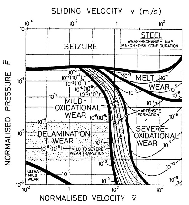
Figure 4: Wear mode map for non-lubricated sliding steel on steel in air at room temperature[3]
What do lubricants do?
The surfaces of most engineering materials have a certain roughness which is indicated in terms of well-defined parameters such as average roughness (Ra), root mean square roughness (RRMS), etc. When two such surfaces start to rub against each other, their roughness peaks and valleys interact and contribute to the overall frictional resistance of the system. One way to reduce friction is by introducing a medium at the contact interface, which ideally would prevent the surfaces from coming in direct contact with each other. In most cases, lubricants are either liquids or semisolids (greases). However, there are numerous applications in which solid lubricants such as graphite, molybdenum disulfide (MoS2), etc. are also used. In extreme cases, lubricants may also have gaseous form, as in the case of air in air bearings.
The primary purpose of lubricants is to reduce friction and wear between two mating surfaces. This is achieved by forming a thin lubricant film which separates the surfaces from coming in direct contact with each other. In addition to friction and or wear reduction, lubricants in many applications also act as heat descriptors, cleaning agents, corrosion inhibitors, etc.
In some cases, the effectiveness of a lubricant can be measured in terms of the frictional response of the system. This is typically done on a measuring instrument called a tribometer. One such method used by tribometers that will be often referred to in the applications section is the Stribeck curve.
How to measure the effectiveness of a lubricant
Tribological properties are system-specific; therefore, tribological tests on tribometers need to be as close to a real-life system as possible. The most important parameters of interest in tribology are the coefficients of friction and wear. However, these parameters need a reference for quantification, such as time, velocity, temperature, contact pressure, etc., or a combination of these. In this section, select test methodologies to study the friction and wear behavior of the system are described.
Friction tests
Stribeck curves
Stribeck curves were originally conceptualized to study the different friction or lubrication regimes of journal bearings. In their simplified form, Stribeck curves depict the coefficient of friction as a function of sliding velocity, see Figure 5. Over the past decades, Stribeck curves have been used in numerous other applications, such as food and beverages, bio-medical applications, inks, etc. To produce Stribeck curves you need a tribometer. The trends in the Stribeck curves can be used to determine the three different lubrication regimes, namely:
- boundary regime
- mixed friction regime
- hydrodynamic regime
The boundary regime, which occurs at the lowest speeds, is characterized by contact between surface asperities as the lubricant cannot entrain into the clearance between the two mating surfaces to form a load-bearing film. Due to direct contact between the surfaces and poor lubrication, the system is prone to wear and high frictional resistance.
As the speed is increased, the system transfers into the mixed friction regime. Due to the increased speed, a small amount of lubricant enters the clearance, just enough to separate the surfaces and minimize asperity contact. This leads to reduced friction and much lower chances of wear.
Finally, in the hydrodynamic regime, also called the fluid friction regime, there is enough lubricant entrained into the contact to form a significant load-bearing fluid film, thereby avoiding the possibility of asperity contact. The increase in frictional resistance is due to the increased film thickness. In this regime, the rheological properties of the lubricant are dominant.
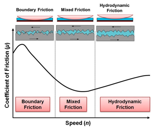
Figure 5: Sketch of a simplified Stribeck curve depicting the coefficient of friction as a function of speed
Extended Stribeck curve
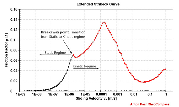
Figure 6: An “extended” Stribeck curve depicting friction in both static and kinetic regimes[5]
Conventional Stribeck curves depict the frictional response of the system in the kinetic regime, in which there is relative motion between the surfaces at macroscopic level. Extended Stribeck curves, on the other hand, extend the conventional Stribeck curves into the static regime. This can be achieved if the tribometer has the capability to set and control forces and displacement in the nano- and micro-scale, in addition to the macro-scale.
In Figure 6, the extended Stribeck curve shows the friction coefficient of the system plotted over 9 orders of magnitude of sliding velocity, starting from almost a nanometer per second. The region of the curve plotted in black represents the static friction regime and that in red is the kinetic regime. The friction at the transition point is the limiting friction of the system.
Extended Stribeck curves reveal a lot of information about the frictional response of the system, both in the static and kinetic regime. One such parameter is the limiting friction of the system. Be it from a torque sweep or the extended Stribeck tests, limiting friction is a very important factor that needs to be considered for many applications. While in some cases a low breakaway friction is desired, as in the case of most engine contacts, there are also cases in which a high value of limiting friction is expected, such as that between the sole of our shoes and the floor. In most cases, though, there is an optimum friction that offers the highest efficiency for the system.
In order to obtain an extended Stribeck curve the tribometer should be able to set and control forces and displacement over a very large range, starting from the nano-scale. As with the breakaway torque tests, the first step in the extended Stribeck tests is to apply the preset normal force and keep the system at the set load for a duration of 5 minutes. This allows some amount of relaxation from the stresses brought about by the applied load. Thereafter, the sliding velocity is logarithmically increased from a very low value (say 10 nm/s) to about 1 m/s. Care should be taken to make sure that the data point duration in the low-speed regime is long enough to let the instrument reach the set velocity. In most cases, the extended Stribeck test is carried out two or three times with the same set of sample/specimen. During the first run, the surfaces of the specimen undergo a phenomenon known as running-in in which they conform with each other either through wear or plastic deformation, or both. It is generally agreed upon that the second and/or third runs offer a more realistic depiction of the frictional behavior of the system.
Limiting friction test

Figure 7: Tribogram showing breakaway torque
The transition from static state to kinetic state of motion occurs in very short time scales and is characterized by micron- or sub-micron-scale relative displacements. One of the many ways to determine this transition is through a torque sweep on a tribometer. Here, after contact is established between the mating surfaces and the preset normal force applied, the system is maintained at the set load for a period of at least 5 minutes for stress relaxation. After this, the torque is logarithmically increased and the sliding distance observed as a function of the applied torque as shown in Figure 7. The breakaway torque is characterized by a sudden and steep increase in the sliding distance for a relatively small increase in the applied torque. The value of torque and the friction coefficient corresponding to the point of inflection are the breakaway torque and the coefficient of limiting friction of the system, respectively. The accuracy in determining the limiting friction of the system depends upon the capability of the tribometer to be able to set and control the forces and displacement.
Read more about the influence of humidity on limiting friction.
Wear tests
There are many kinds of wear measurement methods. They are often referred to by their specific contact arrangements. The most common ones are illustrated in Figure 8.
Both friction and wear measurement results are critically dependent on the different contact arrangements, sliding velocities, contact pressures, and environmental conditions such as temperature and humidity.
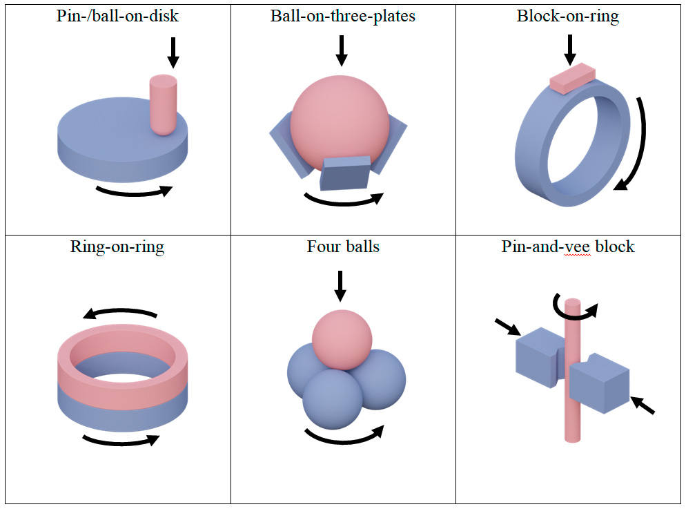
Figure 8: Different wear tests according to their contact geometries
Calculation of wear in the ball-on-disk arrangement
The relevant ASTM standards determine the amount of wear by measuring the appropriate linear dimension of both specimens (ball and disk) or by weighing them before and after the test. The standard ball-on-disk setup is shown in the following figure with the parameters required to calculate wear.
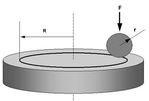
Figure 9: Typical ball-on-disk setup, where F is the normal force applied on the ball, r is the ball radius, and R is the radius of the wear track
Assuming that there is no significant ball or pin wear, the volume loss of the disk is given by the following equation[4]:
$$V_{disk}=2πR[r^2sin^{-1}(d/2r)-(d/4)(4r^2-d^2)^{1/2}]$$
Where:
R = wear track radius
d = wear track width
r = ball radius
Vdisk = disk wear volume
Alternatively, the loss of material from the disk can also be defined by making a profile scanning over the wear track on the disk. Variations around the wear track can be caused by debris and plastic deformation. Therefore, enough profiles should be made to get a representative value. Most profilometer software can readily calculate the area covered by the profile.
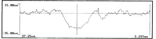
Figure 10: Example of a profile on a wear track
Assuming that there is no significant disk wear, the volume loss of the spherical ball (or a spherical-ended pin) is given by the following equation[3]:
$$V_{ball}=(πh/6)[3d^2/4+h^2]$$
Where:
$h=r-[r^2-d^2/4]^{1/2}$
d = wear scar diameter
r = ball radius
Vball = ball wear volume
The wear factor (wear rate) of the disk and sample could then be calculated as follows:
$$K_{disk}={V_{disk} \over Fl}$$
$$K_{ball}={V_{ball} \over Fl}$$
Where:
Vdisk = wear volume of the disk
Vball = wear volume of the ball
F = normal force
l = total sliding distance
Kdisk = wear factor (wear rate) of the disk
Kball = wear factor (wear rate) of the ball
Other tests
In addition to the tests described above, there are many other test profiles which are used to characterize the tribological behavior of systems. Examples of such tests are temperature sweeps, normal force or contact pressure sweeps, and isothermic or isobaric tests in unidirectional or oscillatory mode. The most important aspect of choosing the right test method is to try and keep the test conditions, including the samples/specimen, as close as possible to the real-life application.
Conclusions
The efficiency and lifespan of tribological interfaces can be improved significantly once their working mechanism is understood. In most cases, it is very expensive, time-consuming, and complicated to investigate real-life systems under their actual operating conditions, and therefore investigations are scaled down in such a way that the tests can be carried out in laboratories on tribometers. The choice of test method, test geometry, and the specimen is very important to be able to apply the results from model tests to the real-life applications.
References
- Jost, P. (1966). Lubrication (Tribology) – A report on the present position and industry’s needs. Department of Education and Science. London, UK: H. M. Stationery Office.
- ASTM G40 Standard Terminology Relating to Wear and Erosion
- Ashby, M. F., Brunton, J. H. and Lim, S. C. (1987). “Wear-Rate Transitions and Their Relationship to Wear Mechanisms”, Acta Metall. 35, pp. 1343–1348.
- ASTM G99 Standard Test Method for Wear Testing with a Pin-on-Disk Apparatus
- Pondicherry, Kartik S. et al., Extended stribeck curves for food samples, Biosurface and Biotribology(2018),4(1):34 dx.doi.org/10.1049/bsbt.2018.0003