Many liquid, gel-like, or semi-solid everyday substances are typically characterized by measuring a sample’s viscosity, flow curve, and yield point using rotational viscometers/rheometers. Water is a typical sample with a low viscosity and has no yield point. Toothpaste on the other hand has a higher viscosity and a yield point. The yield point tells us how much force needs to be applied so that the material starts to flow.This article describes how a flow curve is measured with a rotational viscometer and how the yield point can be calculated.
Flow curve and yield point determination with rotational viscometry
Measurement with a rotational viscometer/rheometer
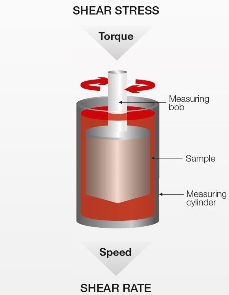
Figure 1: Rotational viscometer: The instrument’s motor turns the measuring bob inside a cup filled with sample.
Most rotational viscometers/rheometers work according to the Searle principle: A motor drives a bob inside a fixed cup. The rotational speed of the bob is preset and produces the motor torque that is needed to rotate the measuring bob. This torque has to overcome the viscous forces of the tested substance and is therefore a measure for its viscosity.
A rotational viscometer measures the dynamic viscosity [ƞ] of a sample. Newton's Law defines the dynamic viscosity η as the shear stress divided by the shear rate[3]. When we measure the viscosity on a rotational viscometer we apply to the sample a certain shear stress or a certain shear rate, respectively.
$\eta = {{\tau} \over {\dot{\gamma}}}$
Equation 1: Newton's viscosity law
$\eta$ ... dynamic viscosity [Pa.s]
$\tau$ ... shear stress [Pa]
${\dot{\gamma}}$ ... shear rate [s-1]
The physical properties speed and torque can be translated into the rheological properties shear rate and shear stress if the measurement is performed using a standard measuring geometry according to ISO 3219[2]. The viscometer’s speed is converted into shear rate using a conversion factor (the factor depends on the measuring geometry used) and the torque is also converted into shear stress using a conversion factor. Usually, this is automatically done by the instrument.
speed × conversion factor = shear rate
torque × conversion factor = shear stress
In a typical rotational test, the shear rate is preset. This means that the viscometer translates the chosen shear rate into speed and measures the resulting torque, which it then translates into shear stress[3].
Such a measurement, where the shear rate is increased and the resulting shear stress is measured, is called a flow curve.
Flow curve
Definition of a flow curve
Typical rotational tests are viscosity functions that depend on shear rate, shear stress, time, or temperature. The results of a rotational test can be displayed on the one hand as a flow curve diagram showing the resulting shear stress values, and on the other hand as the corresponding viscosity function. A measurement on a rotational viscometer/rheometer in which the shear rate is increased step-wise and the respective shear stress is determined for each shear rate is called a flow curve. A material can show different flow behaviors such as ideally viscous, shear-thinning and shear-thickening behavior.
In nearly all production stages the viscosity of food samples has a great impact e.g. in the mixing process of dairy substances and for the generation of new formulations for vegetable sauces. At low shear rates the sample‘s viscosity at rest is measured (e.g. when stored in the bottle) and at high shear rates the sample‘s viscosity in movement (e.g. when swallowing or shaking the sample) is tested. Hazelnut cream for example should have a defined viscosity when it is spread on a slice of bread and should not to be too watery or too thick.
Flow curve measurement

Figure 2: Viscometer/rheometer settings for a flow curve
A flow curve can be generated via predefined settings on the rotational viscometer/rheometer:
- The shear rate is increased step-wise with a defined measurement point duration for each point.
- The temperature and other ambient conditions are constant.
The resulting flow curve shows the shear stress versus the shear rate. Usually, the individual measurement points are connected by lines to show the flow curve.
Flow curve of ideally viscous substances
For ideally viscous or so-called Newtonian samples, the shear stress increases linearly with increasing shear rate. Figure 4 shows such a flow curve of two Newtonian samples, sample (a) being more viscous than sample (b). The samples’ viscosity does not change with increasing shear rate. Typical examples would be olive oil for sample (a) and water for sample (b).
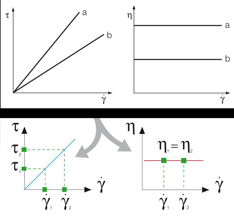
Figure 3: Flow curves of two different ideally viscous fluids
Flow curve of shear-thinning substances
For materials with shear-thinning flow behavior, the gradient of the shear stress decreases at higher shear rates. This means that the sample’s viscosity becomes lower at higher shear rates. This is a typical behavior of many materials from daily life, e.g. cosmetics such as creams and lotions, food samples such as ketchup or molten chocolate, as well as chemical samples such as paints and coatings. See figure 4.

Figure 4: Flow curve of a shear-thinning material

Figure 5: Flow curve of a shear-thickening material
Flow curve of shear-thickening substances
For materials with shear-thickening flow behavior, the gradient of the shear stress increases at higher shear rates. This means that the sample’s viscosity increases at higher shear rates. This is a relatively rare flow behavior, typically seen in samples with a high solid content such as ceramic suspensions, starch dispersions, or dental composites.
Yield point calculation
Definition of the yield point
The yield point (also called yield stress) is the lowest shear-stress value above which a material will behave like a fluid, and below which the material will act like a solid[2].
Typical examples of materials that have a yield point are creams, ketchup, toothpaste, and sealants. The yield point is the minimum force that must be applied to those samples so that they start to flow.
Substances with a yield stress only start to flow once the outside force acting on them is larger than their internal structural forces. Below the yield point, the substance shows “solid-like” behavior. For example, toothpaste does not flow out of its tube if no external force is applied. Below the yield point, it behaves solid-like. The yield point can be overcome by increasing the shear forces (e.g. by pressing on the tube). Above the yield point, the sample flows (out of the tube) and behaves liquid-like.
The yield point is of vital importance for many practical issues and applications, e.g. for quality control of final products or for optimizing the production process.
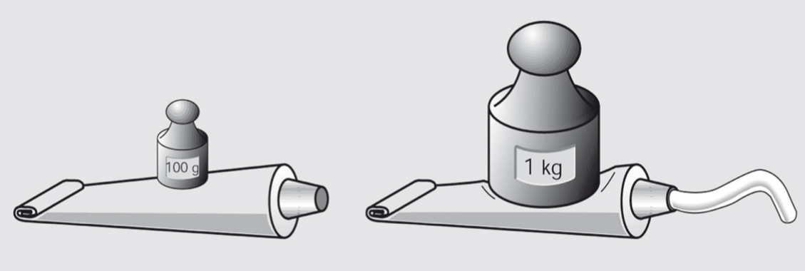
Figure 6: The yield point is the minimum force that must be applied to a sample so that it starts to flow.
Calculation of the yield point with a flow curve
The yield point is not a material constant but depends on the measuring and analysis method used. There are many different methods available. On rotational viscometers/rheometers, the yield point is often calculated from flow curves measured with a linear increase of the shear rate (as described above). The yield point is not measured directly, but calculated using model functions (e.g. Bingham, Casson, or Herschel-Bulkley). For all these approximation models, the yield point value ${\tau}_0$ (spoken "tau zero") is determined by extrapolation of the flow curve towards a low shear rate value. Each different model function usually produces a different yield point because the calculation is different.
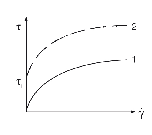
Figure 7: Flow curve of two different shear-thinning materials
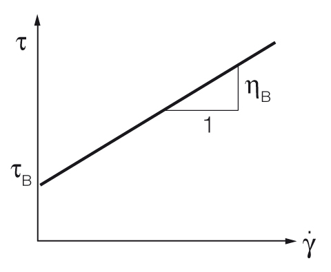
Figure 8: Bingham model for the calculation of the yield point
Bingham yield point calculation
The Bingham regression calculates the yield point with a constant slope[4, 5]. It is mostly used when the material shows a constant slope above the yield stress, for example some types of food or cosmetics. Historically, before the use of computers, it was a very easy way to determine the yield point. See figure 8.
$$\tau = \tau_B + \eta_B \cdot {\dot{\gamma}}$$
Equation 2: Bingham equation for the yield point
$\tau$ ... shear stress [Pa]
$\tau_B$ ... Bingham yield point [Pa]
$\eta_B$ ... Bingham viscosity [Pa.s]
${\dot{\gamma}}$ ... shear rate [s-1]
Casson yield point calculation
For the Casson yield point calculation, curve fitting is performed using a square root function[6]. This takes the curve’s bending into consideration and is therefore often better suited for shear-thinning and shear-thickening materials than the Bingham calculation. It is typically used for food products such as chocolate. See figure 9.
$$\sqrt{\tau} = \sqrt{\tau_c} + \sqrt{\eta_c \cdot \dot\gamma}$$
Equation 3: Casson equation for the yield point
$\tau$ ... shear stress [Pa]
$\tau_c$ ... Casson yield point [Pa]
$\eta_c$ ... Casson viscosity [Pa.s]
$\dot\gamma$ ... shear rate [s-1]
Herschel-Bulkley yield point calculation
The Herschel-Bulkley regression describes the flow curve of a material with a yield stress and shear-thinning or shear-thickening behavior at stresses above the yield stress[7].
$$\tau = \tau_{HB}+ {c} \cdot \dot\gamma^{p}$$
Equation 4: Herschel-Bulkley equation for the yield point
$\tau$ ... shear stress [Pa]
$\tau_{HB}$ ... Herschel Bulkley yield point [Pa]
c ... flow coefficient, also called Herschel Bulkley viscosity [Pa.s]
${\dot\gamma}$ ... shear rate [s-1]
p ... exponent, also called Herschel Bulkley index
$\tau_{HB}$ describes the material’s yield point. c is the so-called “flow coefficient” or “consistency index” that describes the viscosity at a certain shear rate. The parameter p (also called “Herschel-Bulkley index”) describes the material’s flow behavior:
- p < 1: shear-thinning
- p > 1: shear-thickening
- p = 1: Bingham flow behavior
With Herschel-Bulkley, in most cases a better curve fitting will be achieved than with the Bingham model.
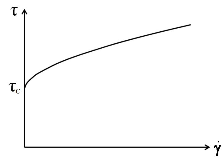
Figure 9: Casson model for the yield point

Figure 10: Herschel-Bulkley model for the yield point
Calculation of the static yield point with the vane technique
The determination of the static yield point using the vane technique is a very quick, easy, and direct method for analyzing the yield point with an entry-level rotational viscometer. This method avoids slipping effects and minimizes structural changes of the sample during immersion of the spindle. For the measurement of the yield point a vane spindle with four to eight thin blades arranged at equal angles is used. By inserting the vane spindle into e.g. a paste-like sample the structure of the sample is disrupted only slightly in comparison to concentric cylinder systems. It is important that the diameter of the beaker is at least twice the size of the vane diameter. A change in the sample’s structure can be further minimized by using the original sample container rather than pouring the sample into a beaker. The yield value strongly depends on the sample preparation and pretreatment of the sample before starting the measurement[8, 9]. To measure the yield point a constant low speed is preset on the rotational viscometer. The maximum yield stress, which can be detected during the measurement, is the yield point value. To illustrate the yield point in a graph the torque is plotted against the time. The diagram has usually three typical regions[10]:
- First, the shear stress increases due to deformation as an elastic response.
- A shear stress peak is achieved due to a collapse of the microstructure of the material. This point is called the yield point.
- Afterwards, a stress decay due to the structural breakdown can be visualized.
")
Figure 11: Static yield point determination with the vane technique (red line represents the yield point)
What is the difference between static and dynamic yield stress? If the yield stress is analyzed from samples where the structure is not disrupted, it is called “static yield stress”. In contrast, if the yield point is analyzed from samples which were pre-sheared before the measurement, it is called “dynamic yield stress”.
Further yield point calculation methods
Many more model functions than described in chapter 3.2 are available for determining the yield point with a flow curve measurement, e.g. Casson/Steiner[11] or Windhab[12]. In practical use, it often depends on the field of application which yield point calculation leads to better results.
Furthermore, the yield point of a material can also be calculated using other rheological measurement methods than those described, for example:
- Logarithmic shear-rate-controlled flow curves performed with rotational viscometers/rheometers
- Linear or logarithmic shear-stress-controlled flow curves performed with rotational viscometers/rheometers
- Amplitude sweeps performed with air-bearing oscillatory rheometers; this method is the most advanced and accurate method available today[3].
Conclusion
It can be summarized that for rotational viscometers/rheometers which work according to the Searle principle, the measuring system rotates at a certain speed, the corresponding torque is measured (or vice versa), and the viscosity is calculated. Furthermore, a flow curve can be measured to analyze the sample’s flow behavior. This is done by increasing the shear rate step by step and determining the respective shear stress for each shear rate. A quick yield point check for quality control purposes with an entry-level viscometer can be carried out using the vane technique. By adjusting the yield point of a sample like ketchup or shower gel, the force that is applied to the tube when pressing it and therefore the force that is needed for the sample to start flowing out can be simulated.