- Basics of rheology
- 3iTT test
- Amplitude sweeps
- Angular Frequency
- Ball Measuring System
- Dynamic Mechanical Analysis
- Evaluation of the time-dependent flow behavior
- Examples of a flow curve and viscosity curve
- Examples of the calculation of shear rates
- Flow curve and yield point determination with rotational viscometry
- Frequency sweeps
- Glass Transition Temperature
- Hooke´s Law
- How to measure viscosity
- Internal structures of samples and shear-thinning behavior
- Log-log diagram
Basics of rheology

Rheology is used to describe and assess the deformation and flow behavior of materials. Fluids flow at different speeds and solids can be deformed to a certain extent. Oil, honey, shampoo, hand cream, toothpaste, sweet jelly, plastic materials, wood, and metals – depending on their physical behavior, they can be put in an order: On the one side liquids, on the other side solids, and in between highly viscous, semi-solid substances.
On this page, the fundamental principles – the basics of rheology – are presented and explained. It is dedicated to giving an introduction to rheology, provides information about measuring geometries and rotational as well as oscillatory tests, and also contains definitions of the most important terms, such as shear stress, shear rate, or shear deformation. You will also find everything there is to know about flow and viscosity curves and examples of calculations and test types.
Learn more
Rheology articles and glossary
- LVE Range
- Methods and devices for controlling the temperature
- Newton's Law
- Powder rheology
- Structural Decomposition and Regeneration
- Structural Strength
- Temperature-dependent behavior (oscillation)
- Temperature-dependent behavior with gel formation or curing
- Temperature-dependent behavior without chemical modifications
- Temperature-dependent flow behavior
- Time-dependent behavior (oscillation)
- Time-dependent behavior with gel formation or curing
- Torsional Tests
- Tribology
- Yield point, evaluation using the flow curve
- Zero Shear Viscosity
Since rheology and viscometry are closely related, why not also have a look at our page dedicated to everything about viscosity and viscometry.
Rheometers
Anton Paar offers a wide range of rheometers to suit different applications and industrial requirements.
Introduction to rheology
Rheology and viscous behavior

Figure 1.1
Rheology is a branch of physics. Rheologists describe the deformation and flow behavior of all kinds of material. The term originates from the Greek word “rhei” meaning “to flow” (Figure 1.1: Bottle from the 19th century bearing the inscription “Tinct(ur) Rhei Vin(um) Darel”. Exhibited in the German Apotheken-Museum [Drugstore Museum], Heidelberg. The term “rhei” indicates that the content of the bottle is liquid.). Rheometry is the measuring technology used to determine rheological properties.
What is viscosity?
All liquids are composed of molecules; dispersions also contain some significantly larger particles. When put into motion, molecules and particles are forced to slide along each other. They develop a flow resistance caused by internal friction.
Larger components present in a fluid are the reason for higher viscosity values.
Why do different substances have different viscosities?
Molecules in fluids come in different sizes: solvent molecules approx. 0.5 nm, polymers approx. 50 nm (coiled ball diameter at rest), and mineral particles approx. 5 µm = 5000 nm. One nanometer (1 nm) equals 10-9 m; one micrometer (1 µm) is equal to 10-6 m. This means that the size ratio between molecules and particles is in the range from 1:100 to 1:10,000 (Figure 1.2). The ratio of 1:1000 can be illustrated with the following figure: The molecules are fish, each of them 10 cm (0.1 m) long, whereas the particles are ships with a length of 100 m (Figure 1.3).
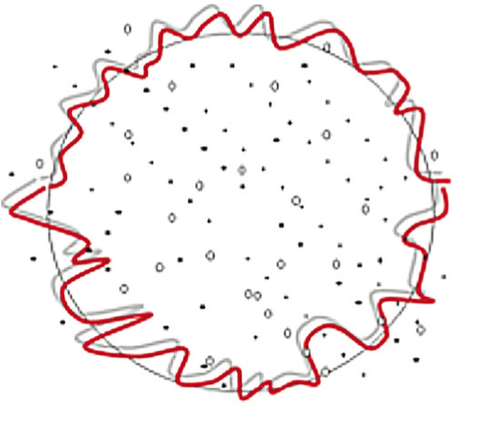
Figure 1.2: Comparison of sizes: solvent molecules (dots), polymer molecules (small circles), and particles (red outline). Viscosity is the internal friction that occurs when all components in a flowing liquid are forced to slide along each other.
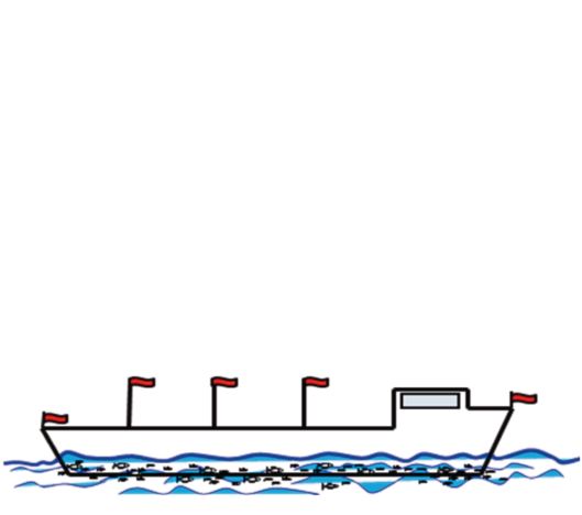
Figure 1.3: Visualization of the size ratio of 1:1000, which is similar to the size ratio of molecules and particles in a fluid. It can be compared with the size difference between small fish and large ships.
Rotational viscometers, oscillatory rheometers, and measuring geometries
Modern rheometers can be used for shear tests and torsional tests. They operate with continuous rotation and rotational oscillation (Figure 2.1). Specific measuring systems can be used to carry out uniaxial tensile tests either in one direction of motion or as oscillatory tests.
With a viscometer, only the viscosity values of a sample can be determined. This can be done by performing rotational tests, mostly speed-controlled, or by using other methods of testing. The results are presented as flow curves or viscosity curves. Find many methods and approaches to measure viscosity in the related Wiki article. Rheometers are able to determine many more rheological parameters.
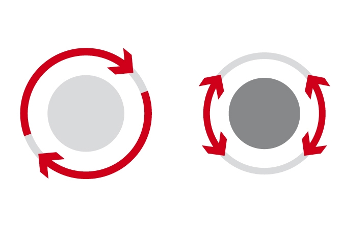
Figure 2.1: Measuring principle of a typical rheometer for rotational tests with continuous rotation (left) or rotational oscillation (right)
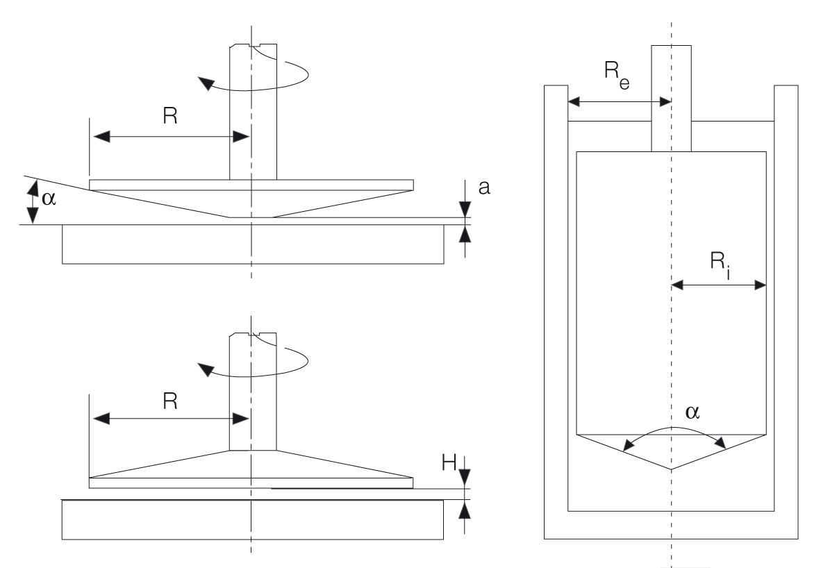
Figure 2.2: Measuring systems: cone-plate (with radius R, cone angle α, truncation a); plate-plate (with radius R, distance between plates H); and concentric cylinders (with bob radius Ri and cup radius Re and internal angle α at the tip of the bob)
Simple methods for measuring viscosity include so-called relative measuring systems. The results obtained are always dependent on the used device and cannot be compared with each other (e.g. flow cups [a,b,c] or falling/rolling ball viscometers[d,e]).
Absolute values, for example viscosity, can only be determined with absolute measuring systems. In contrast to relative values, absolute values do not correlate with the size of the measuring system. They have a relatively narrow shear gap as defined by specific standards for measuring systems such as ISO 3219[f] and DIN 53019[g]. These standards describe the following measuring geometries (Figure 2.2 and 2.3): cone-plate, concentric cylinders and plate-plate.
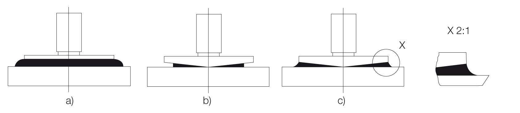
Figure 2.3: Filling of cone-plate measuring system after gap setting: a) overfilled, b) underfilled, c) correct amount (according to DIN 51810-1)
Rotational tests and viscosity
Rotational tests
Rotational tests (Figure 3.1) with a rheometer can be carried out in one of two operation modes, which differ in their preset parameters (Tables 2 and 3). The first way is to present the velocity via rotational speed or shear rate (controlled shear rate, CSR or CR). This simulates processes that are dependent on flow velocity or volume flow rate, such as application of coatings with a brush, or of paints by spraying or flow through a tube (Figure 3.2). The second way is to preset the driving force via torque or shear stress (controlled shear stress, CSS or CS). These tests simulate force-dependent applications, such as the force required to start pumping a material at rest, to squeeze sealing materials out of a cartridge, or paste out of a tube. Conversion of torque into the shear stress and rotational speed into the shear rate, and vice versa, is possible via conversion factors.
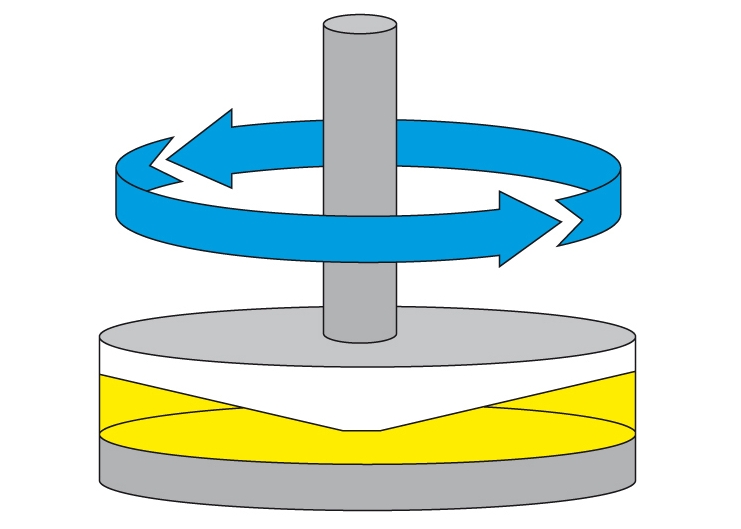
Figure 3.1: Rotational shear test on a sample; the cone rotates while the lower plate is stationary.
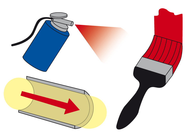
Figure 3.2: Shear-rate-controlled tests can be used to simulate applications that depend on flow velocity and volume flow rate, such as application of coatings with a brush, or of paints by spraying, or flow through a tube.
| Rotation with controlled shear rate (CSR) | Preset test parameters | Result |
|---|---|---|
| Raw data from the rheometer | Rotational speed n (in min⁻¹) | Torque M (in Nm) |
| Rheological parameters, calculated | Shear rate $\dot \gamma$ (in s⁻¹) | Shear stress τ (in Pa) |
| Rotation with controlled shear stress (CSS) | Preset test parameters | Result |
|---|---|---|
| Raw data from the rheometer | Torque M (in Nm) | Rotational speed n (in min⁻¹) |
| Rheological parameters, calculated | Shear stress τ (in Pa) | Shear rate $\dot \gamma$ (in s⁻¹) |
For calculating the viscosity, the type of operation mode is irrelevant because the parameters shear stress and shear rate are both available, either as a preset value or as a result of the test.
CSR and CSS preset profiles for flow curves (Figure 3.3):
- Preset rotational speed or shear-rate ramp, usually ascending or descending in steps
- Preset torque or shear-stress ramp, usually ascending or descending in steps
For shear rates above 1 s-1, a typical setting recommended for both modes is a duration of at least one to two seconds, which is to be maintained for each measuring point because the sample needs a certain time to adapt itself to each shear step.
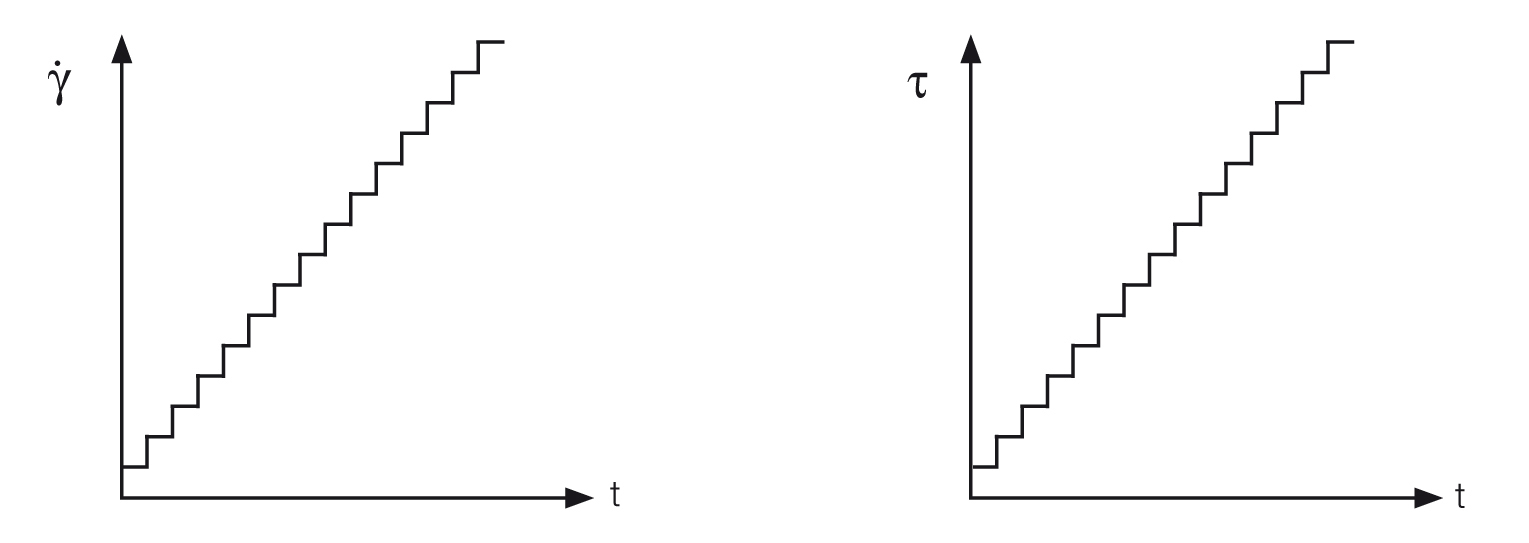
Figure 3.3: Preset profiles for flow curves as time-dependent step-like ramps, here with 15 steps corresponding to 15 measuring points, with controlled shear rate CSR (left) and controlled shear stress CSS (right)
Definition of terms: Shear stress, shear rate, law of viscosity, kinematic viscosity
The two-plates model is used to define the rheological parameters needed for a scientific description of flow behavior (Figures 4.1 and 4.2). Shear is applied to a sample sandwiched between the two plates. The lower stationary plate is mounted on a very rigid support, and the upper plate can be moved parallel to the lower plate. Before calculating the viscosity, it is necessary to first define the shear stress and the shear rate.
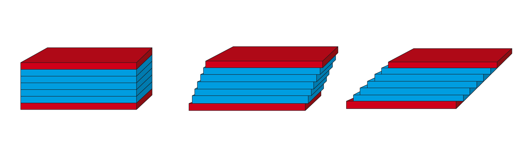
Figure 4.1: Two-plates model for shear tests: Shear is applied to the sample sandwiched between the two plates when the upper plate is set in motion, while the lower plate is stationary. The figure is an idealized illustration of the sample’s individual planar fluid layers, which are displaced in relation to each other[1].
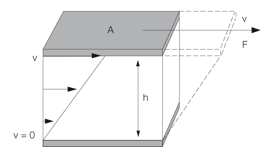
Figure 4.2: Calculation of shear stress and shear rate using the two-plates model with shear area A, gap width h, shear force F, and velocity v
Shear stress
Definition: $\tau$ = F / A with shear stress $\tau$ (pronounced: tau), shear force F (in N, newton) and shear area A (in m2), see Figure 4.3. The unit for shear stress is 1 N/m2 = 1 Pa (pascal). A rheometer records the shear force via the torque at each measuring point.
Shear rate
Definition: $\dot \gamma$ = v / h with shear rate $\dot \gamma$ (pronounced: gamma dot), velocity v (in m/s) and shear gap h (in m), see Figure 4.4. The unit for shear rate is 1/s = 1 s-1, also called reciprocal seconds. A rheometer records the velocity as the rotational speed at each measuring point. The size of the shear gap is also known for the measuring system used. Find examples for calculation of shear rates here.
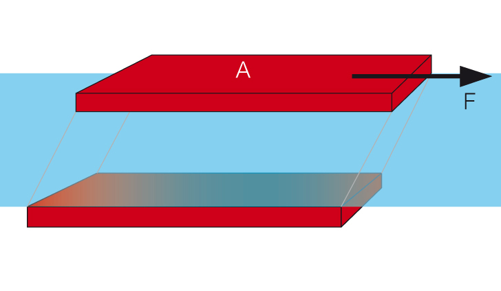
Figure 4.3: Two-plates model used to define the shear stress using the parameters shear force F and shear area A of the upper, movable plate
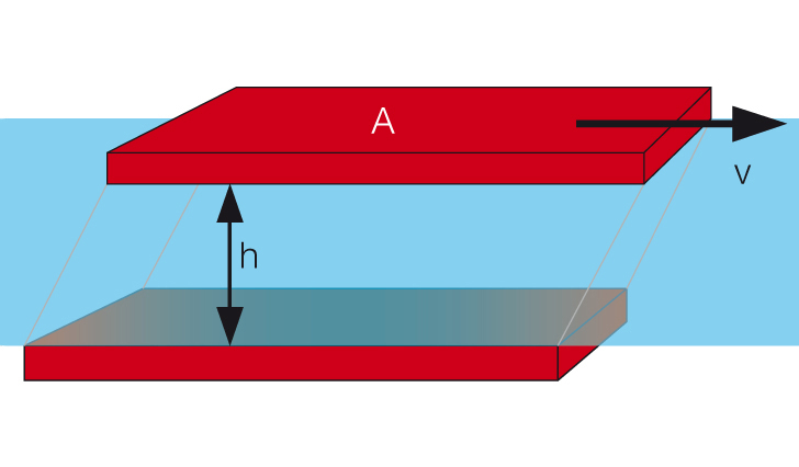
Figure 4.4: Two-plates model used to define the shear rate using the parameters velocity, v, of the upper, movable plate and distance, h, between the plates
Viscosity or shear viscosity / law of viscosity
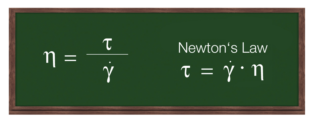
Figure 4.5: The law of viscosity
Definition: $\eta = {\tau\over{\dot{\gamma}}}$ with viscosity η (pronounced: eta), shear stress $\tau$ (in Pa) and shear rate $\dot{\gamma}$ (in s-1), see Figure 4.5 (some viscosity values are displayed in Table 1).
Figure 4.5: The law of viscosity: Viscosity $\eta$ is defined as shear stress $\tau$ divided by shear rate $\dot{\gamma}$ (left). The law of viscosity, here depicted as follows: shear stress $\tau$ is shear rate $\dot{\gamma}$ times viscosity $\eta$ (right).
| Flowing material | Viscosity values |
|---|---|
| Gases/air | 0.01 mPas to 0.02 mPas / 0.018 mPas |
|
Water at 20 °C (at 0 °C/ 40 °C/ 60 °C/ 80 °C/ 100 °C) |
1.0 mPas (1.8 mPas/ 0.65 mPas/ 0.47 mPas/ 0.35 mPas/ 0.28 mPas) |
| Milk, coffee cream | 2 mPas to 10 mPas |
| Olive oil | Approx. 100 mPas |
|
Motor oils (for example SAE 10W-30, at +23 °C/ +50 °C/ +100 °C) |
50 mPas to 1000 mPas (175 mPas/ 52 mPas/ 20 mPas) |
|
Polymer melts (at T = +150 °C to +300 °C and at shear rates of between 10 and 1000 s-1) |
10 mPas to 10,000 Pas |
|
Polymer melts (zero-shear viscosity, which means shear rates below 1 s-1) |
1 kPas to 1 MPas |
| Bitumen at T = +80 °C/ +60 °C/ +40 °C/ +20 °C/ 0 °C | 200 Pas / 1 kPas / 20 kPas / 0.5 MPas / 1 MPas |
All three parameters, namely shear stress, shear rate, and viscosity, can only be precisely measured if there are – as a precondition – laminar flow conditions and there is therefore uniform flow (Figures 4.6 and 4.1). This means that turbulent flow with vortex formation must not occur.
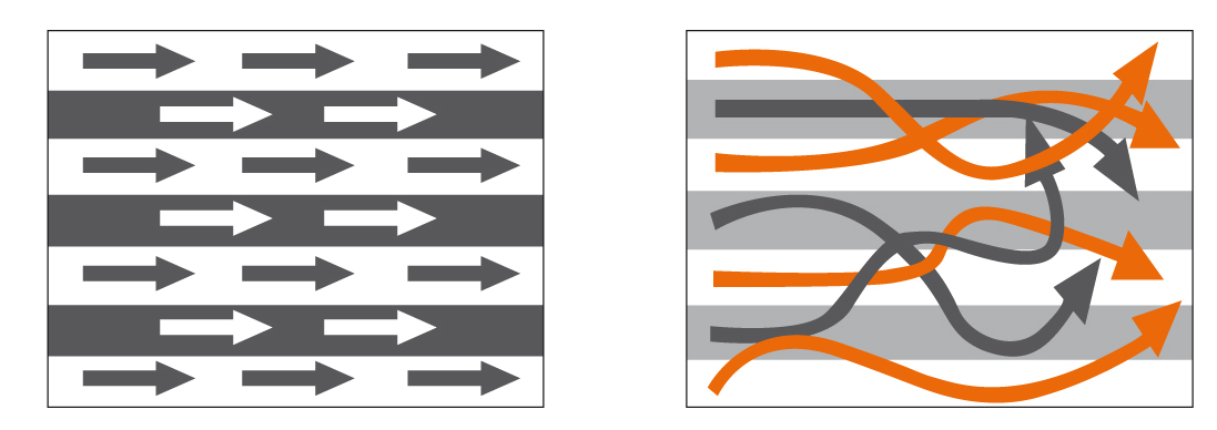
Figure 4.6: Homogenous flow or laminar flow (left) and turbulent flow with vortex formation (right)
Kinematic viscosity
Another type of viscosity is the kinematic viscosity $\nu$ (pronounced: nu).
Definition: $\nu$ = $\eta$ / $\rho$ with shear viscosity η (in Pas) and density ρ (in kg/m3). The unit for kinematic viscosity is m2/s = 106 mm2/s. For calculations, please note: The units for density are kg/m3 and g/cm3, where 1000 kg/m3 = 1 g/cm3.
The unit for shear viscosity is 1 Pas = 1000 mPas (pascal seconds, milli-pascal-seconds). Other units include 1 kPas = 1,000 Pas (kilo-Pas), 1 MPas = 1,000,000 Pas (mega-Pas). A previously used unit was 1 cP = 1 mPas (centipoise, best pronounced in French), but cP is not an SI unit and should not be used any longer.
Kinematic viscosity is always determined if gravitational force or the weight of the sample is the driving force. This applies, for example, to tests with flow cups, falling-ball and capillary viscometers. A previously used unit for the kinematic viscosity was 1 cSt = mm2/s (centistokes), but cSt is not an SI unit and should not be used any longer.
The SI system is the international system of units (French: système international d’unités)[2].
Flow behavior, flow curve, and viscosity curve
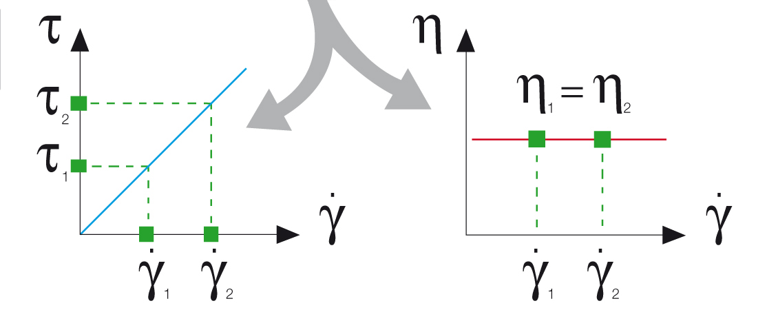
Figure 5.1: The flow curve (left) is obtained by plotting shear stress versus shear rate. Next, the viscosity function is calculated (right).
Viscosity values are not constant values as they are affected by many conditions. The subject of this chapter is flow behavior under shear at constant temperature. Flow behavior can be presented in two types of diagrams (Figure 5.1):
- Flow curves with shear stress $\tau$ and shear rate $\dot \gamma$, usually with the latter plotted on the x-axis
- Viscosity curves with viscosity η and shear rate $\dot \gamma$ (or shear stress $\tau$), usually with the latter plotted on the x-axis. Applying the law of viscosity, each measuring point is calculated as follows: $\eta$ = $\tau$ / $\dot \gamma$
Ideally viscous flow behavior (or: Newtonian flow behavior) means that the measured viscosity is independent of the shear rate (Figure 5.2, line 1). Typical materials from this group include water, mineral oil, silicone oil, salad oil, solvents such as acetone, as well as viscosity standards (e.g. calibration oils).
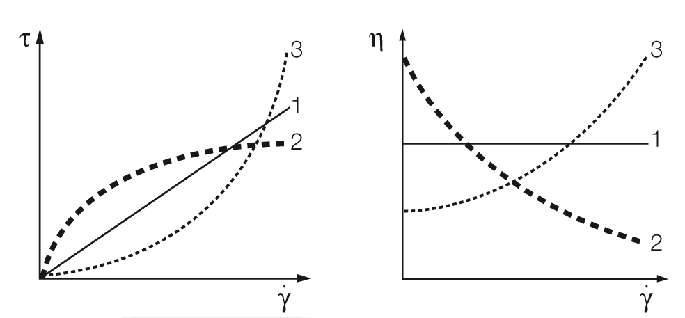
Figure 5.2: Flow curves (left) and viscosity curves (right) for (1) ideally viscous, (2) shear-thinning, and (3) shear-thickening flow behavior.
Shear-thinning behavior (or: pseudoplastic flow behavior) is characterized by decreasing viscosity with increasing shear rates (Figure 5.2, line 2). Typical materials that show this behavior are coatings, glues, shampoos, polymer solutions and polymer melts. Since viscosity is shear-dependent, it should always be given with the shear condition. Example: η1(${\dot \gamma}_1$) = 0.5 Pas (at 10 s-1) and η2(${\dot \gamma}_2$) = 0.1 Pas (at 100 s-1). Shear-thinning behavior is related to the internal structures of samples.
Shear-thickening (or: dilatant flow behavior) means increasing viscosity with increasing shear rates (Figure 5.2, line 3). Materials that typically display such behavior include highly filled dispersions, such as ceramic suspensions (casting slurries), starch dispersions, plastisol pastes that lack a sufficient amount of plasticizer, dental filling masses (dental composites) as well as special composite materials for protective clothing.
For evaluating behavior in the low shear-rate range, it is beneficial to use a log-log plot for the diagrams of flow curves and viscosity curves. The advantage of diagrams on a logarithmic scale is that a very large range of values (several orders of magnitude) can be illustrated clearly in one diagram. Often the biggest changes in viscosity just take place within the range of low shear rates, which is below $\dot \gamma$ = 1 s-1. With a presentation on a linear scale, however, this range can only be depicted to a limited extent.
Approaches to measuring viscous behavior
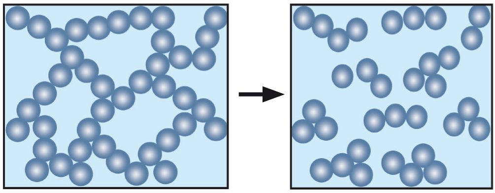
Figure 6.1: When at rest, the interacting forces between particles form a stable, three-dimensional network. The material is in a solid state (left). After the yield point has been exceeded, the superstructure breaks down and the material may start to flow (right).
The yield point is the lowest shear-stress value above which a material will behave like a fluid, and below which the material will act like a – sometimes very soft – solid matter (according to prEN ISO 3219-1). The yield point or yield stress is the minimum force that must be exceeded in order to break down a sample’s structure at rest, and thus make it flow.
A sample’s superstructure can be imagined as being a stable, three-dimensional, consistent, physico-chemical network of forces interacting between the individual components of the sample; for example, between the particles of a rheology additive in a dispersion (Figure 6.1). Click here for more details and procedures on yield point evaluation.
For evaluating time-dependent flow behavior, shearing is kept constant. For test programs with several intervals, this applies to each individual interval. To investigate time-dependent behavior, it is recommended that a step test is carried out, in this case as a rotational test with three intervals.This measurement is usually performed as a time-dependent controlled-shear-rate test:
- Interval (1) Very low shear to simulate behavior at rest at a preset low shear rate
- Interval (2) Strong shear to simulate structural breakdown of the sample during processing at a preset high shear rate, for example when applying paint with a brush or by spraying
- Interval (3) Very low shear to simulate structural regeneration at rest after application using the same preset low shear rate as in the first interval.
See an application example of the behavior of a brush coating before, during, and after application (Figure 6.2).
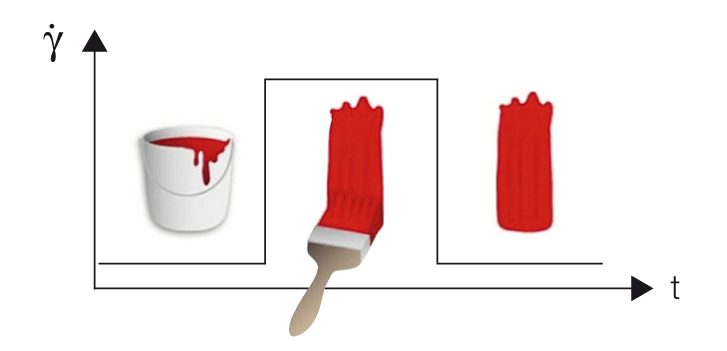
Figure 6.2: Preset profile for a step test with three intervals used to evaluate the behavior of a brush coating: (1) constant low shear rate as in the state at rest, (2) constant high shear rate as applied in a coating process, and finally (3) the same shear rate as in the first interval during structural regeneration at rest after application.

Figure 6.3: Typical temperature-dependent behavior of a sample, here honey, which becomes softer and thinner when heated[1].
Methods for evaluating time-dependent structural regeneration (according to DIN spec 91143-2) can be found here. In contrast, other materials show no structural regeneration, but gel formation or curing under constant shear conditions.
For evaluating temperature-dependent flow behavior, shearing is kept constant. Also, a time-dependent temperature profile is preset. As a result, the function of the temperature-dependent viscosity is usually analyzed. The temperature gradient in the test chamber surrounding the sample should be as small as possible. There are different methods and devices available for controlling the temperature.
Typical tests in this field are used for investigating temperature-dependent behavior without chemical modifications, e.g. softening or melting behavior of samples when heated; or solidification, crystallization, or cold gelation when cooled (Figure 6.3). Other common tests investigate the temperature-dependent behavior during gel formation or chemical curing.
Oscilliation tests and viscoelasticity
Viscoelastic behavior
Many materials display a mixture of viscous and elastic behavior when sheared (Figure 7.1). This is called viscoelastic behavior. The following section deals with typical effects caused by viscoelastic behavior, with special attention paid to the elastic portion:

Figure 7.1: Here are four materials lined up, from left to right: water as an ideally viscous liquid, hair shampoo as an example of a viscoelastic liquid, followed by a viscoelastic solid, such as hand cream, and the Eiffel Tower as an example of an ideally elastic solid made of metal.
Often the elastic portion of the viscoelastic behavior is comparably more pronounced under the following conditions:
- Faster movements, which mean a higher rate of deformation or shear rate, or a higher oscillation frequency
- Lower temperatures: In both cases, the molecular networks will be less flexible and stiffer. The slower the motion and/or the higher the temperature, the more flexible and mobile the behavior of the molecules will be. It is therefore often not sufficient to determine the viscosity alone (with a viscometer) because, in many processes, pronounced elastic effects may occur. This mixture of viscous flow behavior and elastic deformation behavior is known as viscoelastic behavior.
Definition of terms: Shear strain or shear deformation, shear modulus, law of elasticity
The two-plates model is used for the definition of the rheological parameters that are needed for a scientific description of deformation behavior (Figure 8.1). The sample is subjected to shear while sandwiched between two plates, with the upper plate moving and the lower plate being stationary.
Shear stress
Definition: $\tau$ = F / A with shear stress $\tau$ (pronounced: tau), shear force F (in N) and shear area A (in m2), see Figures 8.2 and 8.3. The unit for shear stress is N/m2 = Pa (pascal).
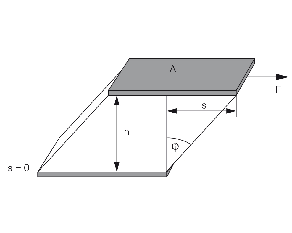
Figure 8.1 Two-plates model for shear tests with shear area A, gap width h, shear force F, deflection path s, and deflection angle ϕ for the calculation of shear stress, and shear strain or shear deformation.
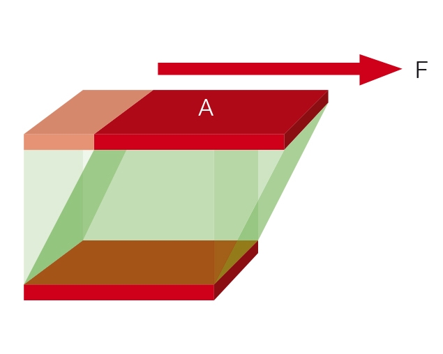
Figure 8.2: Two-plates model used to define the shear stress using the parameters shear force F and shear area A of the upper, movable plate.
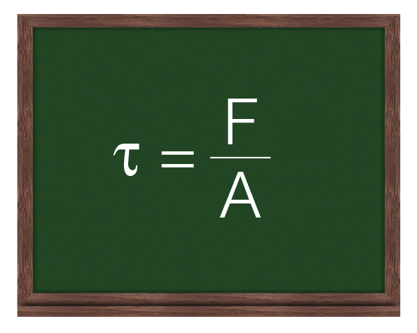
Figure 8.3: Shear stress $\tau$ is defined as shear force F divided by shear area A.
Shear strain or shear deformation
Definition: γ = s / h with shear strain γ (pronounced: gamma), deflection path s (in m), and shear gap h (in m), see Figure 8.4. The unit for shear deformation is (m/m) = 1, which means that deformation is dimensionless. Usually, the value is stated as a percentage.
Shear modulus
Definition: G = τ / γ with shear modulus G, shear stress τ (in Pa), and shear strain or shear deformation γ (with the unit 1).
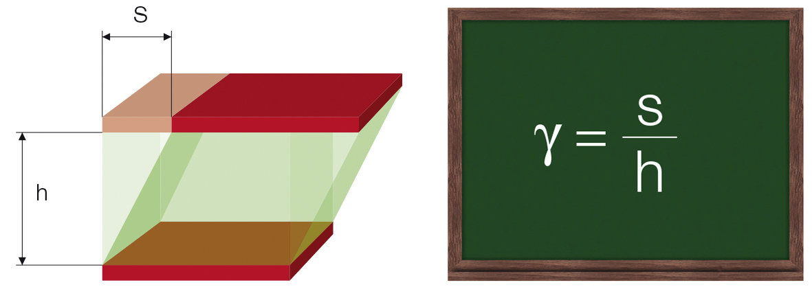
Figure 8.4: Two-plates model used to define the shear strain using the parameters deflection path s of the upper, movable plate, and distance h between the plates (left). Shear strain γ is defined as deflection path s divided by shear gap width h (right).
The unit for shear modulus is Pa (pascal). Other units are: 1 kPa (kilo-pascal) = 1000 Pa, 1 MPa (mega-pascal) = 1000 kPa = 106 Pa, and 1 GPa (giga-pascal) = 1000 MPa = 106 kPa = 109 Pa. The higher the G value, the stiffer the material. The law of elasticity can be compared with the law of springs: F / s = C, with spring force F, deflection path s, and spring constant C, which describes the stiffness of a spring.
Approaches to measuring viscoelastic behavior
The two-plates model can also be used for explaining oscillatory tests (Figure 9.1). A sample is sheared while sandwiched between two plates, with the upper plate moving and the lower plate remaining stationary. A push rod mounted to a driving wheel moves the upper plate back and forth parallel to the lower plate, as long as the wheel is turning. At constant rotational speed, the model operates at a correspondingly constant oscillating frequency.
The deflection path of the upper, movable plate is measured and rheologically evaluated as strain or deformation $\gamma$. When the driving wheel moves, the strain plotted versus time results in a sine curve with the strain amplitude $\gamma_A$ (Figure 9.2).
Parameters for oscillatory tests are usually preset in the form of a sine curve. For the two-plates model, as described above, the test is a controlled sinusoidal strain test. A sine curve is determined by its amplitude (maximum deflection) and its oscillation period. The oscillation frequency is the reciprocal of the oscillation period (Figure 9.3).
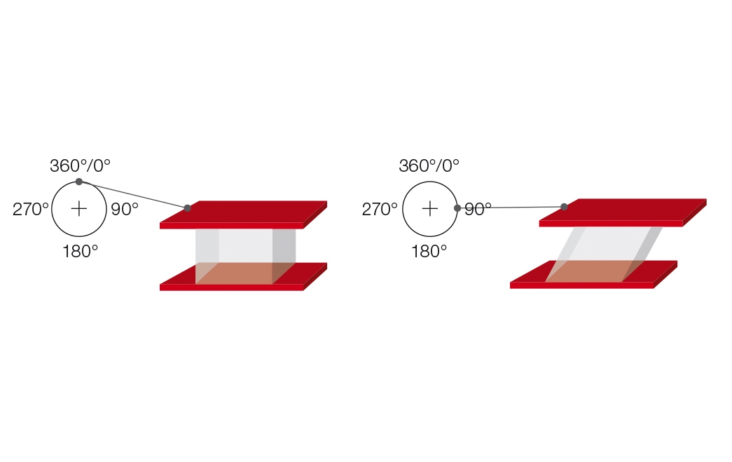
Figure 9.1: Oscillatory test illustrated by the use of the two-plates model with driving wheel and push rod for shear tests. The deflection of the upper plate at the angle positions 0° / 90° / 180° / 270° / 360° of the rotating wheel is shown[1].
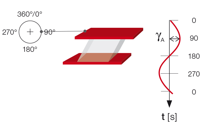
Figure 9.2: Oscillatory test using the two-plates model; on the right: time-dependent strain value with the amplitude γA of the upper plate. Presented over the time axis, a complete sine curve is the result of a full turn of the driving wheel.
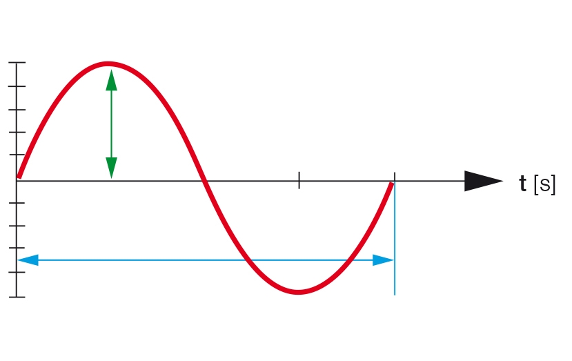
Figure 9.3: A sine curve is described by its amplitude (maximum deflection) and its oscillation period or frequency.
In addition the force that acts upon the lower, stationary plate is measured. This force is required as a counter force to keep the lower plate in position. The signal is rheologically evaluated as shear stress $\tau$. If the sample is not strained by too large a deformation, the resulting diagram over time is a sinusoidal curve of the shear stress with the amplitude $\tau_A$. The two sine curves, i.e. the preset as well as the response curve, oscillate with the same frequency. However, if too large a strain were to be preset, the inner structure of the sample would be destroyed, and the resulting curve would no longer be sinusoidal.
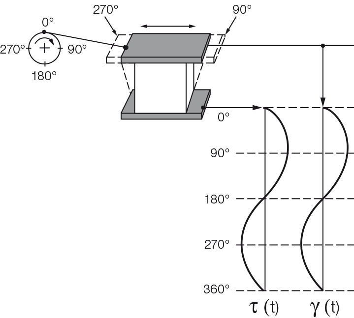
Figure 9.4: Oscillatory test with the two-plates model, here for ideally elastic behavior. There is no time lag between the time-dependent sine curves of the preset shear strain $\gamma$ and the resulting shear stress $\tau$.
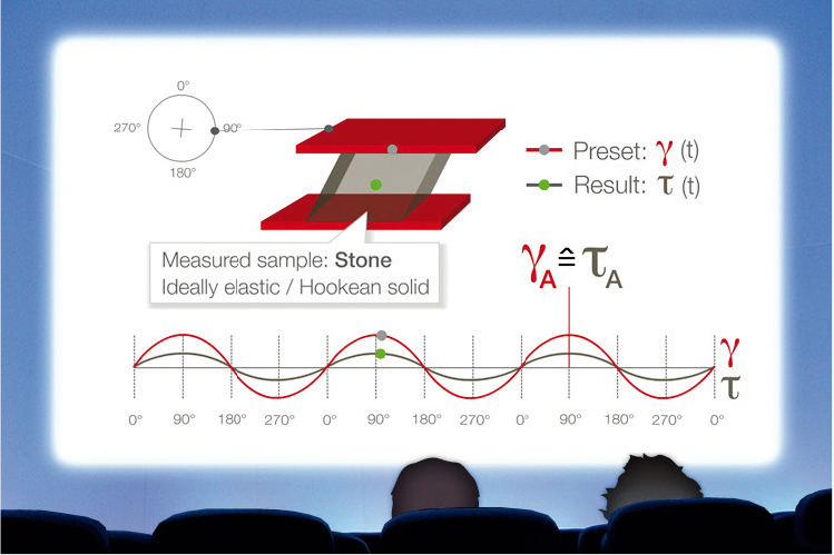
Figure 9.5: With ideally elastic behavior, the sine curves of shear strain γ and shear stress τ do not show any phase shift; the two curve functions reach the amplitude values and the zero crossings at the same time[1].
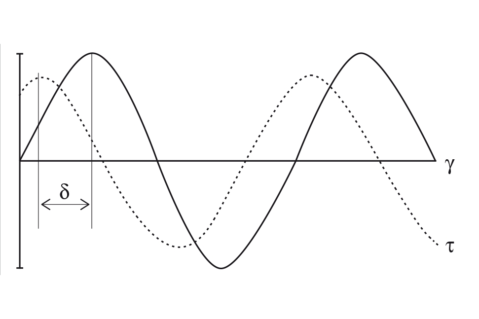
Figure 9.6: Oscillatory test for viscoelastic behavior, presented as a sinusoidal function versus time: For example, with preset shear strain γ and resulting shear stress τ. The two curves are offset by phase shift δ.
For a completely rigid sample, such as one made of steel or stone with ideally elastic behavior, there is no time lag between the preset and the response sine curve (Figures 9.4 and 9.5). Most samples show viscoelastic behavior. In this case, the sine curves of the preset parameter and the measuring result show a time lag for the response signal. This lag is called the phase shift δ (pronounced: delta, Figures 9.6 and 9.7). It is always between 0° and 90°.
For the fluid state, the following holds: The phase shift is between 45° and 90°, thus 90° ≥ δ > 45°. In this case, the material at rest is fluid. The following holds for the phase shift: δ = 0° for ideally elastic deformation behavior and δ = 90° for ideally viscous flow behavior (Figure 9.8). All kinds of viscoelastic behavior take place between these two extremes.
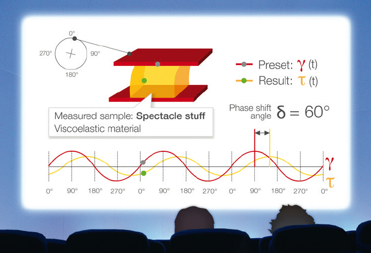
Figure 9.7: For viscoelastic behavior, the sine curves of shear strain γ and shear stress τ show a phase shift, as can be seen from the time lag between the two amplitude values[1]
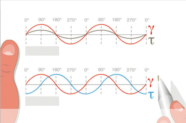
Figure 9.8: Direct comparison of ideally elastic behavior (top) with no phase shift between the preset and response sine curves, and ideally viscous behavior (bottom) with 90° phase shift between the two curves
For the solid, gel-like state, δ is between 0° and 45°: i.e., 45° > δ ≥ 0°. In this case, the material at rest is solid, such as pastes, gels, or other stiff, solid matter. Examples are hand creams, sweet jelly, dairy puddings, and tire rubber.
Complex shear modulus G*
Definition of the law of elasticity for oscillatory shear tests:
G* = τA / γA
with complex shear modulus G* (G star, in Pa), shear-stress amplitude τA (in Pa), and strain amplitude γA (dimensionless, or expressed in %). G* describes the entire viscoelastic behavior of a sample and is called the complex shear modulus G*.
Storage modulus G' and loss modulus G''
The phase shift δ, which is the time lag between the preset and the resulting sinusoidal oscillation is determined for each measuring point. This angle, always between 0° and 90°, is now placed below the G* vector (Figure 9.9).
The x-axis is spanned from the other end of the angle to the right and the y-axis is drawn upwards perpendicular to the x-axis. The part of the G* value that runs along the x-axis is the elastic portion of the viscoelastic behavior presented as G' while the part of the G* vector that is projected onto the y-axis is the viscous portion G''. This means that the complete vector diagram is a presentation of G* and δ, as well as of G' and G'' (Figure 9.10).
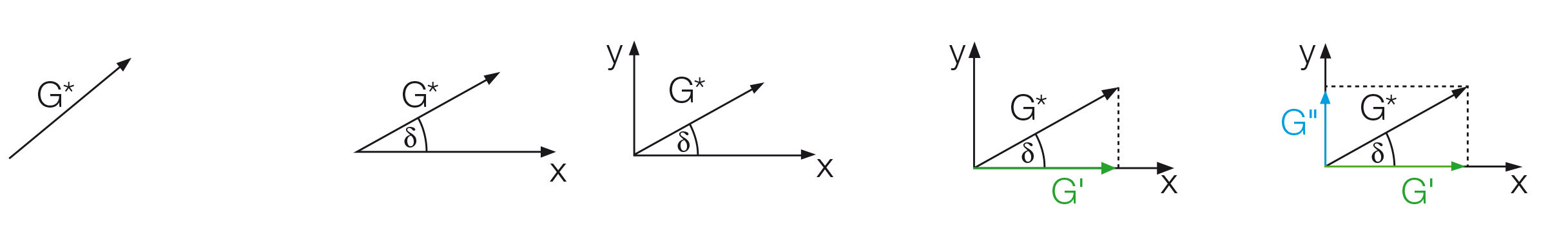
Figure 9.9: Development of a vector diagram in five steps using the following parameters: (1) Vector length as the total amount of the complex shear modulus G*, (2) phase-shift angle δ defining the position of the x-axis, (3) perpendicular y-axis, (4) division of G* into the portions G' on the x-axis and (5) G'' on the y-axis.
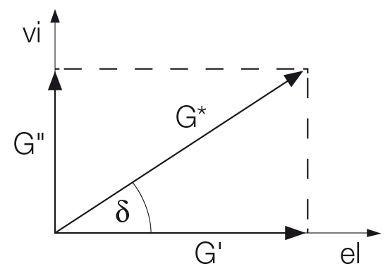
Figure 9.10: Vector diagram illustrating the relationship between complex shear modulus G*, storage modulus G' and loss modulus G'' using the phase-shift angle δ. The elastic portion of the viscoelastic behavior is presented on the x-axis and the viscous portion on the y-axis.
The storage modulus G' (G prime, in Pa) represents the elastic portion of the viscoelastic behavior, which quasi describes the solid-state behavior of the sample. The loss modulus G'' (G double prime, in Pa) characterizes the viscous portion of the viscoelastic behavior, which can be seen as the liquid-state behavior of the sample.
Viscous behavior arises from the internal friction between the components in a flowing fluid, thus between molecules and particles. This friction always goes along with the development of frictional heat in the sample, and consequently, with the transformation of deformation energy into heat energy. This part of the energy is absorbed by the sample; it is used up by internal friction processes and is no longer available for the further behavior of the sample material. This loss of energy is also called energy dissipation.
In contrast, the elastic portion of energy is stored in the deformed material; i.e. by extending and stretching the internal superstructures without overstressing the interactions and without overstretching or destroying the material.
When the material is later released, this unused stored energy acts like a driving force for reforming the structure into its original shape.
Storage modulus G' represents the stored deformation energy and loss modulus G'' characterizes the deformation energy lost (dissipated) through internal friction when flowing. Viscoelastic solids with G' > G'' have a higher storage modulus than loss modulus. This is due to links inside the material, for example chemical bonds or physical-chemical interactions (Figure 9.11).
On the other hand, viscoelastic liquids with G'' > G' have a higher loss modulus than storage modulus. The reason for this is that, in most of these materials, there are no such strong bonds between the individual molecules (Figure 9.12).
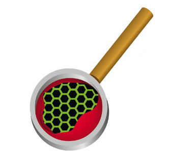
Figure 9.11: Viewed through a magnifying glass: Viscoelastic solids predominantly consist of chemically bonded molecules, or structures with other strong interaction forces.

Figure 9.12: Viewed through a magnifying glass: Viscoelastic liquids are typically composed of mainly unlinked individual molecules, which may show some entanglement as, for example, uncrosslinked polymers.
Loss factor or damping factor: tan δ = G''/ G'
(tangent delta), unit: dimensionless or 1. This factor describes the ratio of the two portions of the viscoelastic behavior. The following applies (see also the vector diagram in Figure 9.10):
- For ideally elastic behavior δ = 0°. There is no viscous portion. Therefore, G'' = 0 and with that tan δ = G''/ G' = 0.
- For ideally viscous behavior δ = 90°. There is no elastic portion. Therefore, G' = 0 and thus the value of tan δ = G''/ G' approaches infinity because of the attempt to divide by zero.
In some diagrams, the loss factor tan δ is plotted in addition to the curves of G' and G'', in particular if there is a phase transition in the sample. This is also called the sol/gel transition point or simply the gel point. It means that the character of the sample has changed during the measurement from the liquid or sol state to the solid or gel state and vice versa. Usually, for practical applications, a liquid is called ideally viscous if tan δ > 100:1 = 100, while a solid material is called ideally elastic if tan δ < 1:100 = 0.01
Amplitude sweeps generally aim at describing the deformation behavior of samples in the non-destructive deformation range and at determining the upper limit of this range (Figure 9.14). Often, it is also interesting to characterize behavior that occurs if this upper limit is exceeded with increasing deformation, when the inner structure gets softer, starts to flow, or breaks down in a brittle way.
Frequency sweeps generally serve the purpose of describing the time-dependent behavior of a sample in the non-destructive deformation range. High frequencies are used to simulate fast motion on short timescales, whereas low frequencies simulate slow motion on long timescales or at rest. In frequency sweeps (Figure 9.15), the oscillation frequency is increased or decreased step-wise from one measuring point to the next while keeping the amplitude constant.
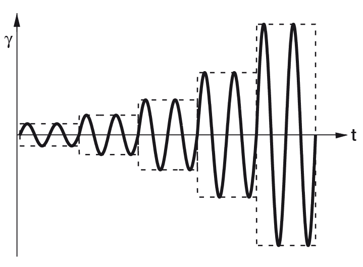
Figure 9.14: Preset of an amplitude sweep: Here, with controlled strain and an increase in the amplitude in five steps. Frequency is kept constant at all five measuring points.
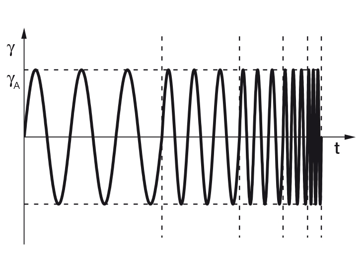
Figure 9.15: Preset of a frequency sweep, here with controlled shear strain and an increase or decrease in frequency in five steps. The strain amplitude γA is kept constant over all five measuring points.
For evaluating time-dependent viscoelastic behavior, oscillatory tests are performed with shearing under constant dynamic-mechanical conditions. This means: Both amplitude and frequency are kept constant for each individual test interval. This is also the case for the evaluation of the temperature-dependent viscoelastic behavior. It is only the temperature that changes according to a preset profile. As a result, the temperature-dependent functions of G' and G'' are usually analyzed.
Conclusion
Liquids with viscous behavior and solids with elastic behavior represent the beginning and end of all possible rheological behavior. Rheology is the science for describing the viscous, viscoelastic, and elastic properties of different materials and how they can be influenced by:
- external forces (or shear stress)
- extent of deformation (or shear strain)
- strain velocity (or shear rate)
- duration of shearing (and in the case of thixotropic behavior, possibly also the duration of the subsequent period of rest)
- temperature (e.g. from T = -150 °C to +1600 °C).
Beyond that, there are many more rheological parameters that can affect rheological behavior. Special measuring instruments and equipment are available, if needed. Examples of further influences on rheological behavior: environmental pressure (e.g. overpressure up to 1000 bar = 100 MPa), magnetic field or electric field strength, UV light rays (ultraviolet) with controlled intensity.
More information can be found in the textbook[3] on which this Wiki, and related sub-topics, are based or other textbooks for further reading [4, 5, 6]. If you are interested in a seminar or a training, order eLearning courses[1] or visit the Anton Paar events and seminars.

Applied Rheology – with Joe Flow on Rheology Road
Are you ready for a journey of discovery down Rheology Road with Joe Flow? This comprehensive resource in Applied Rheology is great for beginners and experienced users alike, and includes insights as well as practical tips for making meaningful measurements from rheology expert Thomas G. Mezger, author of The Rheology Handbook.